Zhenjue tutorial : Différence entre versions
m |
m (→Download) |
||
| (Une révision intermédiaire par un autre utilisateur non affichée) | |||
| Ligne 7 : | Ligne 7 : | ||
==Download== | ==Download== | ||
| − | + | You can find this dataset at <code>https://micmac.ensg.eu/data/zhenjue_dataset.zip</code> <br> | |
Once you have downloaded it, you have to unzip the ".zip" archive. | Once you have downloaded it, you have to unzip the ".zip" archive. | ||
Version actuelle en date du 14 juillet 2022 à 20:19
Sommaire
Description
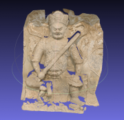
This dataset contain images with different focal length (24 and 100 mm). The purpose of this tutorial is to reconstruct each statue independently (warrior and musician). We will show two methods to reconstruct object in 3D by image geometry (Malt and PIMs).
Download
You can find this dataset at https://micmac.ensg.eu/data/zhenjue_dataset.zip
Once you have downloaded it, you have to unzip the ".zip" archive.
Tutorial
1. Relative orientation
As all MicMac process, the pipeline begin by calling the tool Tapioca to detect tie points :
mm3d Tapioca All ".*JPG" 1500
For this dataset, image have different focal length, so we have to compute first a orientation for the 24mm focal length images.
mm3d Tapas RadialStd ".*JPG" Focs=[20,30] Out=F24
Check residual and number of points used per images.
We use the 24mm orientation as an entry for our command in order to indicate to MicMac there is different focal length :
mm3d Tapas RadialStd ".*JPG" InOri=F24 Out=All
We will now generate a sparse cloud to visualize the relative orientation.
mm3d AperiCloud ".*JPG" All
2. Dense correlation in image geometry (old method)
For this part and the rest of this tutorial, we will focus only on the warrior. Define a mask for dense correlation can be done with the command SaisieMasqQT. Here we define a image mask :
mm3d SaisieMasqQT "DSC_3128.JPG"
The previous tool for dense correlation was Malt. Here we are working in image geometry.
mm3d Malt GeomImage "DSC_313[2-9].JPG" All Master=DSC_3135.JPG ZoomF=4 AffineLast=0
We can compute a dense cloud with the command Nuage2Ply :
mm3d Nuage2Ply NuageImProf_STD-MALT_Etape_6.xml Attr=../DSC_3135.JPG RatioAttrCarte=4 Out=../Warrior.ply
3. Dense correlation in image geometry (new method)
Define a mask for dense correlation can be done with the command SaisieMasqQT. Here we define a 3D mask :
mm3d SaisieMasqQT "DSC_3128.JPG"
The new tool C3DC doesn't need a image master for 3D reconstruction :
mm3d C3DC BigMac "DSC_313[2-9].JPG" All ZoomF=4
4. Comparison
So let's compare the files "Warrior_Malt.ply" and "C3DC-BigMac.ply".
5. Compute a depth map
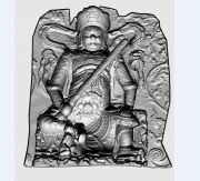
To visualize the depth map, we have to use the tool GrShade to the most elevate resolution map (Z_Num6... here) :
cd MM-Malt-Img-DSC_3135
mm3d GrShade Z_Num6_DeZoom4_STD-MALT.tif ModeOmbre=IgnE Mask=AutoMask_STD-MALT_Num_5.tif FZ=2 Out=../ShadeWarrior.tif
Go further
mm3d SaisieMasqQT DSC_3128.JPG
mm3d Malt GeomImage "DSC_31((2[5-9])|(3[0-1])).JPG" Toutes Master=DSC_3128.JPG ZoomF=4
cd MM-Malt-Img-DSC_3128
mm3d GrShade Z_Num6_DeZoom4_STD-MALT.tif ModeOmbre=IgnE Mask=AutoMask_STD-MALT_Num_5.tif FZ=2 Out=../ShadeMusician.tif
mm3d Nuage2Ply NuageImProf_STD-MALT_Etape_6.xml Attr=../DSC_3128.JPG RatioAttrCarte=4 Out=../Musician.ply
Conclusion
Unfortunately, the tools C3DC and PIMs don't have a radiometric egalisation module. So for instance, if you want to use it in orthophotos or dense cloud, you can still use the old pipeline (Malt,Nuage2Ply,Tawny etc...)

